A complete worked example

Run this once before the bootcamp. It walks the same path as every exercise you will do at the event: measure a baseline → train an agent → evaluate honestly → look at it.

Steps 1–3 take about ten minutes. Step 4 starts a half-hour training run, so kick it off and come back to it — the figures and video below are from exactly that run, so you can read the rest while yours trains.

The task is Pendulum-v1: swing an under-powered pendulum upright and keep it there. It is a continuous-control problem — the agent outputs a torque, not a button press — which makes it a much better rehearsal than CartPole.

Rewards are negative here

Pendulum's reward is a cost: roughly $-(\text{angle}^2 + \text{small terms})$. The best possible return is near 0, and every episode is exactly 200 steps. Closer to zero is better. Do not be alarmed by large negative numbers.

The three scripts live in examples/ in this repository.

---

Step 1 — What does random look like?

Before training anything, find out what you are trying to beat.

conda activate rlbootcamp
python examples/01_random_agent.py

episode  0  steps  200  return  -1146.8
episode  1  steps  200  return  -1289.6
...
Random policy over 20 episodes:
  mean return :  -1202.3
  std         :    284.2
  best / worst:   -750.6 / -1723.9

Two things worth noticing straight away:

• Every episode is exactly 200 steps. The episode ends by truncated, never terminated — there is no "failure" state to fall into, only a time limit.
• The standard deviation is large (±284 on a mean of −1202). Any claimed improvement smaller than that spread is noise, not progress.

Open examples/01_random_agent.py. It is 40 lines and it is the entire Gymnasium API — worth reading before you move on.

---

Step 2 — Train an agent

python examples/02_train.py

This trains SAC for 20,000 steps and writes everything to runs/sac_Pendulum-v1_<timestamp>/.

This takes about 5–10 minutes

On the machine these numbers came from it ran at ~60 steps/second and took 5 minutes 32 seconds. That is normal. SAC performs a gradient update on every environment step, so it is compute-bound rather than simulation-bound.

This is your first honest taste of RL's cost: several minutes for a task you could hand-code in twenty lines. Real problems take hours or days.

While it runs, SB3 prints a table every few episodes:

---------------------------------
| rollout/           |          |
|    ep_len_mean     | 200      |
|    ep_rew_mean     | -326     |   <-- watch this climb toward zero
| time/              |          |
|    fps             | 60       |
|    total_timesteps | 20000    |
| train/             |          |
|    actor_loss      | 41.8     |
|    critic_loss     | 0.65     |
---------------------------------

rollout/ep_rew_mean is the number to watch. The losses are not. Unlike supervised learning, a falling loss in RL does not mean improvement — the critic is chasing a moving target, so its loss can rise while the policy gets better. Judge by return.

Try the other algorithm

python examples/02_train.py --algo ppo --timesteps 100000

PPO is on-policy and needs far more environment steps to reach the same place. Running both is the cheapest way to feel the sample-efficiency difference the algorithm table describes.

---

Step 3 — Evaluate against the baseline

python examples/03_evaluate.py runs/sac_Pendulum-v1_<timestamp>/model.zip

Pendulum-v1 — 20 episodes

  policy                    mean return       std
  ----------------------------------------------
  random baseline               -1321.7     254.4
  agent (stochastic)             -136.8      91.8
  agent (deterministic)          -156.3      92.5

  agent - random = +1165.5

This is what a real result looks like. Note what the script does for you, and why:

• The baseline is printed alongside the agent, always. A number on its own is not a result. Here the agent improves on random by ~1165 — many times the baseline's own standard deviation, so the effect is unambiguous.
• Both action modes are reported. They agree closely (−137 vs −156), which says the learned policy is fairly deterministic already.
• Evaluation uses a different seed from training (--seed 100). Evaluating on your training seeds measures memorisation.

Now go and break it

The example is more instructive when it fails. Try --timesteps 2000 and watch the agent fail to beat random. Try two different --seed values at full length and compare — the spread between seeds is exactly why one run is never enough.

---

Step 4 — Now train it properly

20,000 steps produces an agent that clearly beats random but still wobbles. To see one that essentially solves the task, give it five times the budget:

python examples/02_train.py --timesteps 100000

This one takes about half an hour

The run below took 29 minutes 37 seconds at ~56 steps/second. Start it and go and do something else — that is the honest rhythm of RL work.

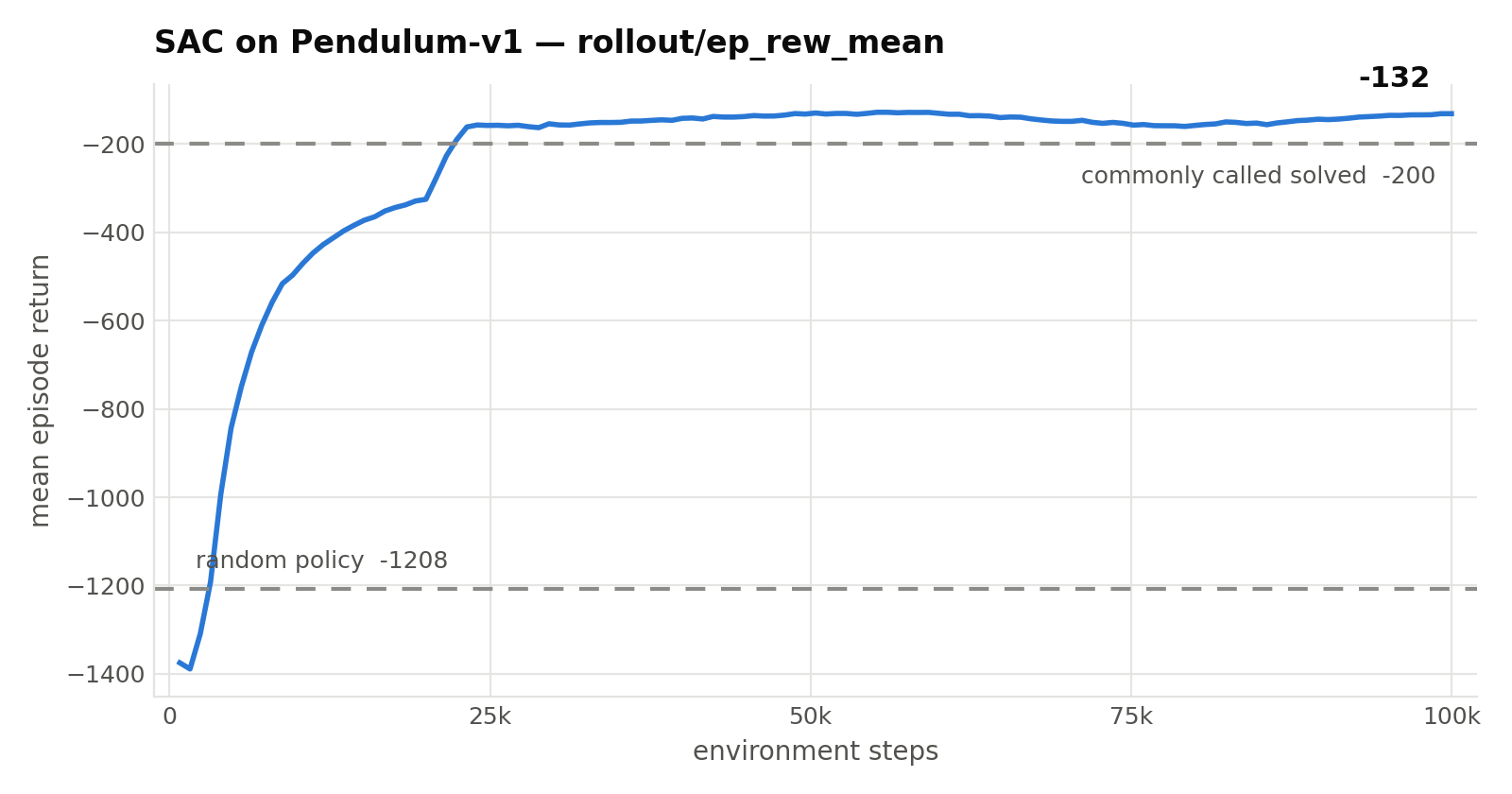
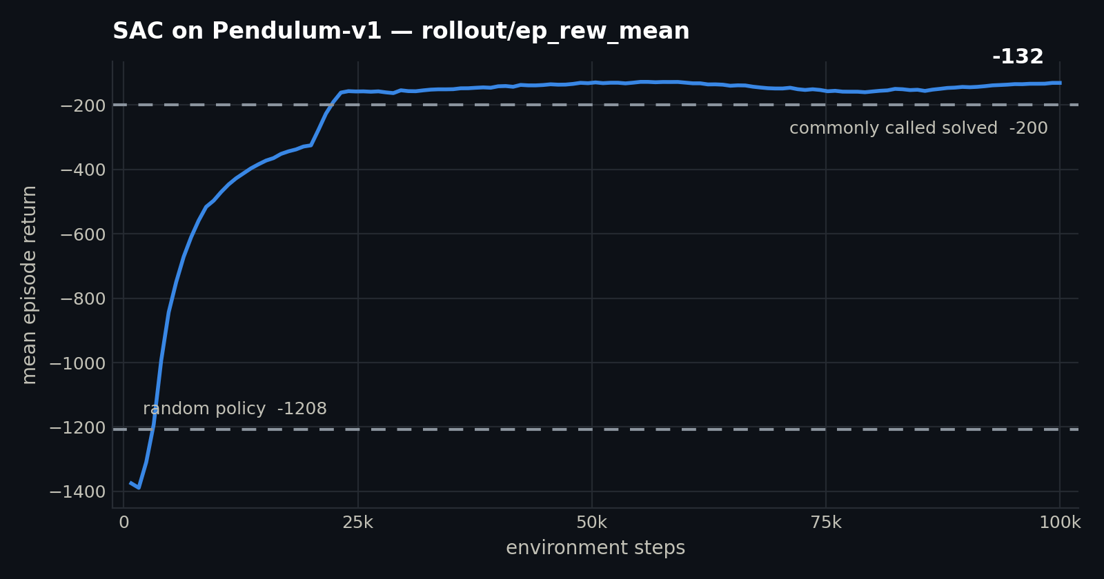
Here is that run's actual learning curve, straight from its TensorBoard logs:

Read it the way you would read your own:

• It starts at the random baseline. The curve's left edge (≈ −1390) sits near the dashed random-policy line, exactly as it should — an untrained policy is a random one.
• Almost all the learning happens in the first 25k steps. It crosses the −200 line — the threshold conventionally called solved for this task — at roughly 23,000 steps, then spends the remaining 75,000 refining.
• The plateau is not flat, and that is normal. It wanders between about −130 and −165 forever. That wobble is the noise floor, and it sets the resolution of any comparison you make: a "gain" of 20 points here is indistinguishable from nothing.
• It never reaches zero. It cannot. The pendulum starts in a random position each episode and takes time to swing up, and every step spent not upright costs reward. Perfect play still scores well below zero — which is why an absolute number means nothing without a baseline beside it.

The diagnostics, and why you should ignore them

The same run's train/* scalars:

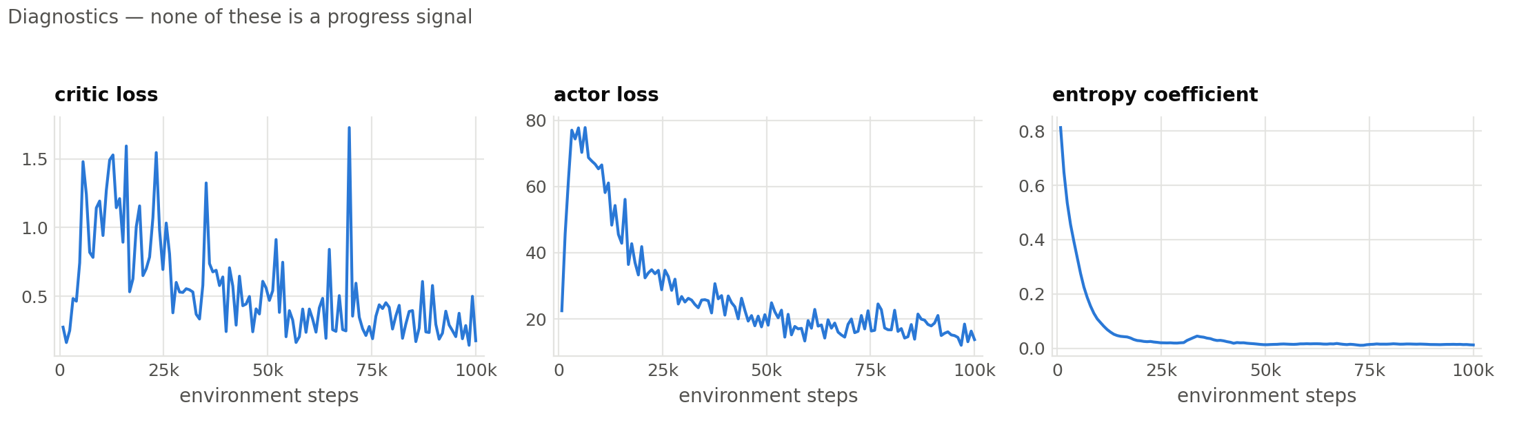
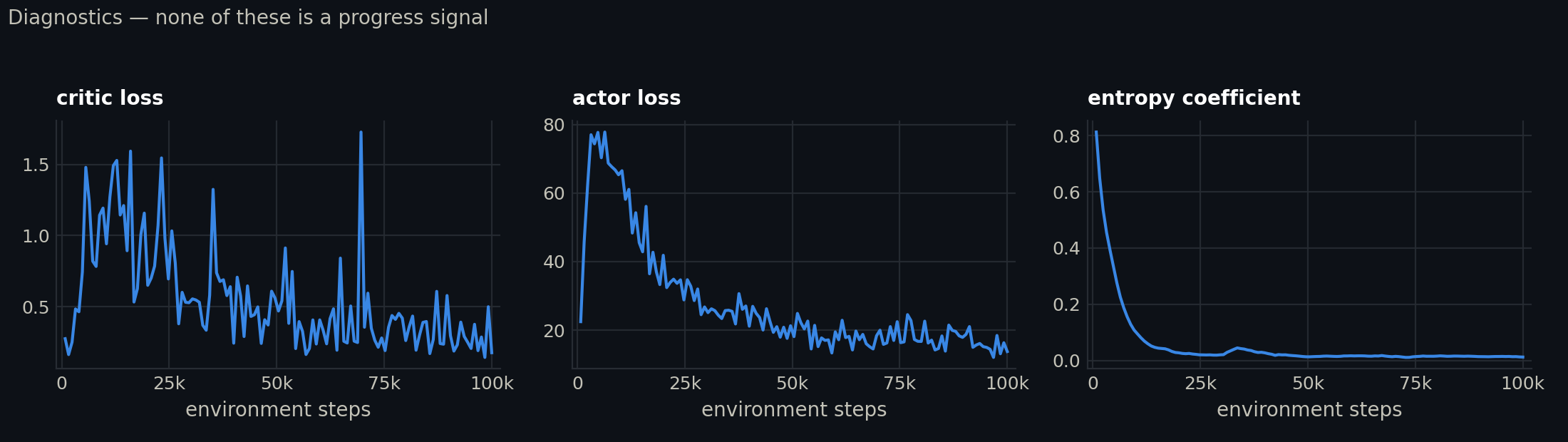
Look at critic loss. The agent went from useless to solved during this run, and the critic loss did not fall in any clean way — it spikes hardest around 25k, precisely when the policy was improving fastest. In supervised learning that pattern would mean something was badly wrong. Here it means the critic is chasing a target that keeps moving because the policy keeps changing.

Actor loss is not an error either; for SAC it is roughly the negative of the critic's opinion of the policy, so it can drift anywhere.

The entropy coefficient is the one with a readable story: SAC tunes it automatically, and its decay from 0.8 to near zero is the agent shifting from exploring to exploiting. Had it collapsed within the first few thousand steps, that would be a genuine warning — exploration died before the agent found anything.

None of these three tells you whether training is working. The return curve does. See TensorBoard for the full panel-by-panel guide, and run it yourself on this data:

tensorboard --logdir runs/
# open http://localhost:6006

And the numbers

Pendulum-v1 — 20 episodes

  policy                    mean return       std
  ----------------------------------------------
  random baseline               -1366.3     245.3
  agent (stochastic)             -165.9      51.5
  agent (deterministic)          -142.0      92.3

  agent - random = +1224.3

Compare against the 20k run from Step 3 (−156.3): five times the training budget moved the deterministic score by about 14 points, while the run-to-run spread is ±92. The longer run is not measurably better on this metric. It is more reliably good — the plateau shows it stopped improving around 25k — but if you reported "100k beats 20k" from these two numbers, you would be reporting noise. This is what needing several seeds looks like in practice.

---

Step 5 — Watch it

Numbers tell you whether it works. Video tells you how — and quite often reveals that the agent found something you did not intend.

python examples/03_evaluate.py runs/sac_Pendulum-v1_<timestamp>/model.zip --video

The .mp4 lands in runs/.../videos/. This needs ffmpeg and pygame; if it fails, see troubleshooting.

Here is the agent from the 100k run above — one full episode, 200 steps:

Watch what it actually does. The agent applies coordinated left-and-right torque corrections, alternating to kill the pendulum's momentum while driving it toward vertical. The corrections shrink in amplitude as it closes on equilibrium — in the render, the torque arrow gets visibly smaller each time — and by roughly one second in, about 30 of the 201 frames, the pendulum is upright and the arrow has disappeared entirely.

It then holds that position for the remaining 85% of the episode at essentially zero action. That is the signature of a genuinely converged control policy: not fighting to stay up, but having found the state where no input is needed and settling into it.

You can read the reward function straight off that behaviour. Pendulum's reward is roughly -(angle² + 0.1 × angular_velocity² + 0.001 × torque²) — three penalties: being off-vertical, moving fast, and using torque. The policy you are watching minimises all three in that order of importance: correct the angle, damp the velocity, then stop spending torque. Nobody wrote that sequence down. It fell out of maximising the sum.

One episode is one sample — same trap as one seed

This episode happens to start about 45° from vertical, which is a kind starting position: the agent can correct straight to upright. Pendulum randomises the initial angle, so on an episode that starts hanging near the bottom you will see something quite different — the motor is too weak to lift the weight directly, so the agent must first swing back and forth to build up energy before it can come up at all.

Both are the same policy. If you watch one clip and conclude "it never needs to swing up," you have made exactly the error the evaluation section warns about, in video form. Render a few episodes before you describe what your agent does.

So here is that same policy given the hardest possible start — hanging straight down, at rest. You can force it rather than waiting for the random draw to hand it to you:

python examples/03_evaluate.py runs/sac_Pendulum-v1_<timestamp>/model.zip \
    --video --start-hanging --video-name pendulum-swingup

Hanging at rest is the bottom of the potential well: minimum potential energy, zero kinetic energy, and a stable equilibrium — left alone, it stays there forever. Upright is the opposite, a potential maximum that is unstable: the smallest error grows. The task is to move the system from the comfortable minimum to the precarious maximum and then hold it there, using a motor too weak to simply lift the weight.

Watch what the policy does about that. It cannot climb directly, so it drives the pendulum back and forth in resonance with its own swing, adding a little energy on each pass — roughly two full swings, out to horizontal and beyond — until it has enough to carry over the top. Then, at exactly the right moment, it stops adding energy and switches to catching the pendulum, converting the swing-up into the same shrinking-correction balance you saw in the first clip. From about frame 60 onward it is upright and still.

That switch is the interesting part. There is no "swing up now, balance later" flag anywhere in the code — no phase variable, no mode selector, no reward term for either behaviour. A single continuous policy produces two qualitatively different strategies because they are what maximises the same reward from two different states. This is what people mean when they say RL discovers control laws rather than being told them.

It also costs what you would expect. This episode returned −330 against the −132 of the lucky start — the swing-up spends real reward getting there. Neither number is the policy's "true" score; the average over many random starts is, which is precisely why 03_evaluate.py reports 20 episodes rather than showing you one.

That is the appeal of RL in one clip, and the warning attached to it: the agent optimises what you wrote, not what you meant. Here the two coincided. When they do not, you get an agent that scores brilliantly while doing something useless — and its reward curve will look just as healthy as the one above.

---

What to take from this

If you can do the following, you are ready:

• Explain what terminated and truncated mean, and why they differ.
• Say why the random baseline is printed next to every result.
• Point at ep_rew_mean rather than a loss when asked if training is working.
• Explain why one seed is not a result.
• Recognise that reward going up is not the same as the task being solved.

That last one is the thread running through the whole bootcamp.

---

Next: TensorBoard →